This is a vignette describing usage of mascarade to
generate masks for clusters on 2D dimensional reduction plots like UMAP
or t-SNE.
Package installation
The package stable version can be installed from CRAN:
install.packages("mascarade")The most recent development version of the package can be installed from GitHub:
remotes::install_github("alserglab/mascarade")Loading necessary libraries
##
## Attaching package: 'data.table'
## The following object is masked from 'package:base':
##
## %notin%Example run
Loading example data from PBMC 3K processed with Seurat (see below for more details).
data("exampleMascarade")UMAP coordinates:
head(exampleMascarade$dims)## UMAP_1 UMAP_2
## AAACATACAACCAC -4.232792 -4.152139
## AAACATTGAGCTAC -4.892886 10.985685
## AAACATTGATCAGC -5.508639 -7.211088
## AAACCGTGCTTCCG 11.332233 3.161727
## AAACCGTGTATGCG -7.450703 1.092022
## AAACGCACTGGTAC -3.509504 -6.087042Cluster annotations:
head(exampleMascarade$clusters)## AAACATACAACCAC AAACATTGAGCTAC AAACATTGATCAGC AAACCGTGCTTCCG AAACCGTGTATGCG
## Memory CD4 T B Memory CD4 T CD14+ Mono NK
## AAACGCACTGGTAC
## Memory CD4 T
## 9 Levels: Naive CD4 T Memory CD4 T CD14+ Mono B CD8 T FCGR3A+ Mono NK ... PlateletExpression table for several genes:
head(exampleMascarade$features)## MS4A1 GNLY CD3E CD14 FCER1A FCGR3A
## AAACATACAACCAC -0.4110536 -0.4081782 1.0157094 -0.393789 -0.1373491 -0.4507969
## AAACATTGAGCTAC 2.5965712 -0.4081782 -0.9189074 -0.393789 -0.1373491 -0.4507969
## AAACATTGATCAGC -0.4110536 0.7526607 0.8148764 -0.393789 -0.1373491 -0.4507969
## AAACCGTGCTTCCG -0.4110536 -0.4081782 -0.9189074 -0.393789 -0.1373491 1.1300704
## AAACCGTGTATGCG -0.4110536 2.3958265 -0.9189074 -0.393789 -0.1373491 -0.4507969
## AAACGCACTGGTAC -0.4110536 -0.4081782 1.1029222 -0.393789 -0.1373491 -0.4507969
## LYZ PPBP CD8A
## AAACATACAACCAC -0.11104505 -0.1416271 2.1039769
## AAACATTGAGCTAC 0.06112027 -0.1416271 -0.3537211
## AAACATTGATCAGC 0.07833934 -0.1416271 -0.3537211
## AAACCGTGCTTCCG 1.40875149 2.9255239 -0.3537211
## AAACCGTGTATGCG -0.97272094 -0.1416271 -0.3537211
## AAACGCACTGGTAC -0.06309661 -0.1416271 -0.3537211Let’s plot these data:
data <- data.table(exampleMascarade$dims,
                   cluster=exampleMascarade$clusters,
                   exampleMascarade$features)
ggplot(data, aes(x=UMAP_1, y=UMAP_2)) +
    geom_point(aes(color=cluster)) +
    coord_fixed() +
    theme_classic()
Now let’s generate cluster masks:
maskTable <- generateMask(dims=exampleMascarade$dims,
                          clusters=exampleMascarade$clusters)
The maskTable is actually a table of cluster borders. A
single cluster can have multiple connected parts, and one a single part
can contain multiple border lines (groups).
head(maskTable)## UMAP_1 UMAP_2 part group cluster
## <num> <num> <char> <char> <fctr>
## 1: -2.581865 -7.829109 Memory CD4 T#1 Memory CD4 T#1#1 Memory CD4 T
## 2: -2.570402 -7.806183 Memory CD4 T#1 Memory CD4 T#1#1 Memory CD4 T
## 3: -2.581865 -7.783258 Memory CD4 T#1 Memory CD4 T#1#1 Memory CD4 T
## 4: -2.593327 -7.771795 Memory CD4 T#1 Memory CD4 T#1#1 Memory CD4 T
## 5: -2.616253 -7.760332 Memory CD4 T#1 Memory CD4 T#1#1 Memory CD4 T
## 6: -2.639179 -7.748869 Memory CD4 T#1 Memory CD4 T#1#1 Memory CD4 TNow we can use this table to draw the borders with
geom_path (group column should be used as the
group aesthetics):
ggplot(data, aes(x=UMAP_1, y=UMAP_2)) +
    geom_point(aes(color=cluster)) +
    geom_path(data=maskTable, aes(group=group)) +
    coord_fixed() +
    theme_classic()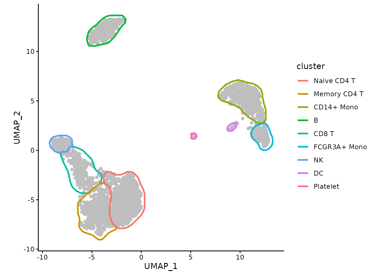
Or we can color the borders instead of points:
ggplot(data, aes(x=UMAP_1, y=UMAP_2)) +
    geom_point(color="grey") +
    geom_path(data=maskTable, aes(group=group, color=cluster), linewidth=1) +
    coord_fixed() +
    theme_classic()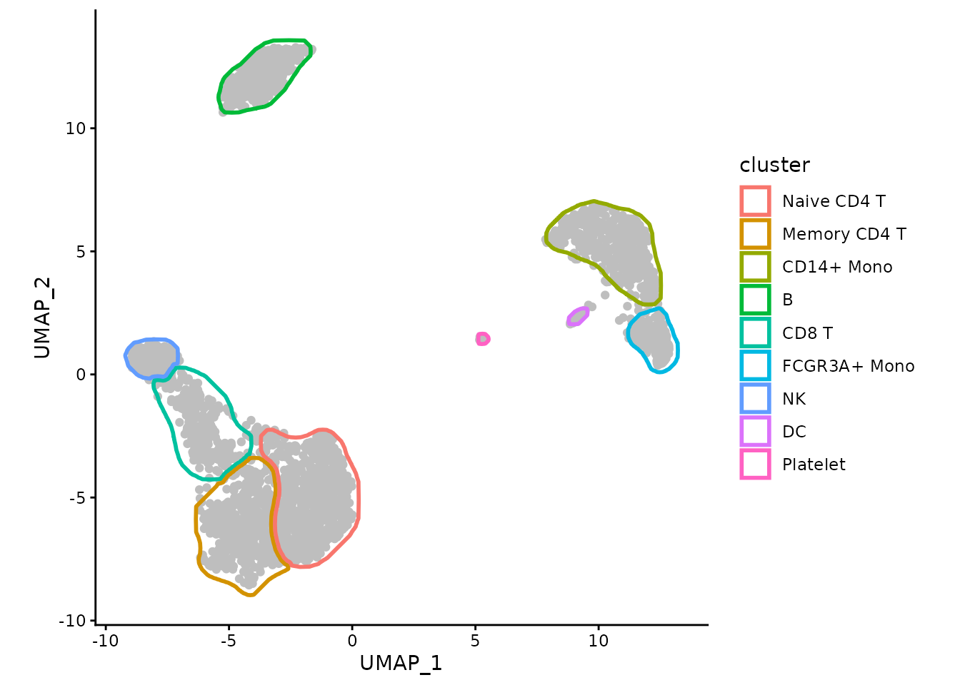
We can use ggforce package to make the borders touch
instead of overlap:
ggplot(data, aes(x=UMAP_1, y=UMAP_2)) +
    geom_point(color="grey") +
    ggforce::geom_shape(data=maskTable, aes(group=group, color=cluster),
                        linewidth=1, fill=NA, expand=unit(-1, "pt")) +
    coord_fixed() +
    theme_classic()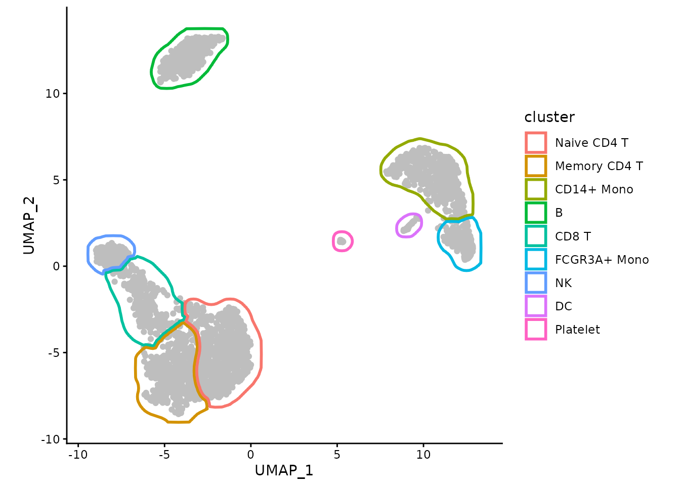
In the presence of small clusters it can help to expand the borders a bit further away from the points.
maskTable <- generateMask(dims=exampleMascarade$dims,
                          clusters=exampleMascarade$clusters,
                          expand=0.02)
ggplot(data, aes(x=UMAP_1, y=UMAP_2)) +
    geom_point(color="grey") +
    ggforce::geom_shape(data=maskTable, aes(group=group, color=cluster),
                        linewidth=1, fill=NA, expand=unit(-1, "pt")) +
    coord_fixed() +
    theme_classic()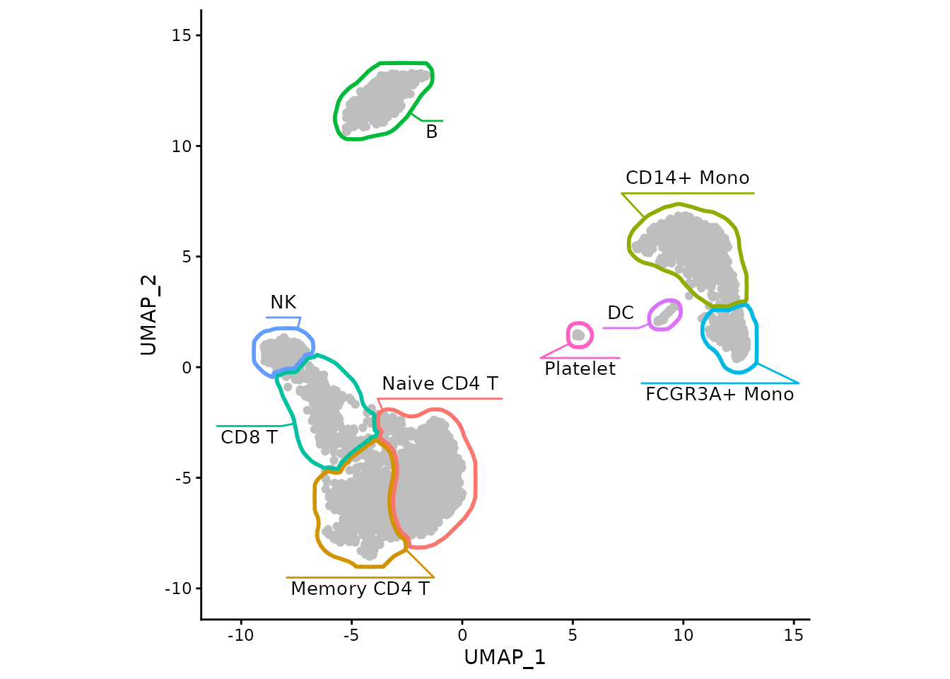
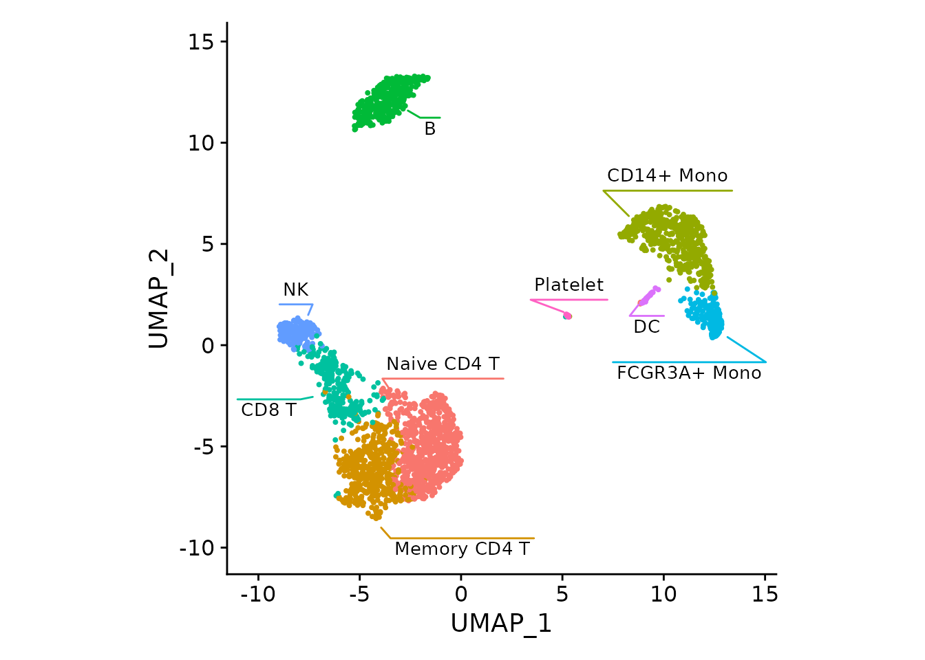
With the help of ggforce-based function
geom_mark_shape we can also put the labels within the plot
itself.
myMask <- list(
    geom_mark_shape(data=maskTable, aes(group=cluster, color=cluster, label = cluster),
                    fill = NA,
                   linewidth=1, expand=unit(-1, "pt"),
                   con.cap=0, con.type = "straight",
                   label.fontsize = 10, label.buffer = unit(0, "cm"),
                   label.fontface = "plain",
                   label.minwidth = 0,
                   label.margin = margin(2, 2, 2, 2, "pt"),
                   label.lineheight = 0,
                   con.colour = "inherit",
                   show.legend = FALSE),
    # expanding to give a bit more space for labels
    scale_x_continuous(expand = expansion(mult = 0.1)),
    scale_y_continuous(expand = expansion(mult = 0.1))
)

ggplot(data, aes(x=UMAP_1, y=UMAP_2)) +
    geom_point(color="grey") +
    myMask +
    coord_fixed() +
    theme_classic()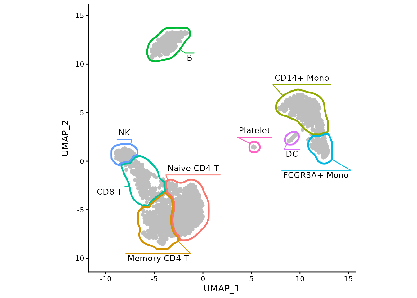
The same can be achived with the fancyMask() helper
function:
ggplot(data, aes(x=UMAP_1, y=UMAP_2)) +
    geom_point(color="grey") +
    fancyMask(maskTable, ratio=1, cols = scales::hue_pal()) +
    theme_classic()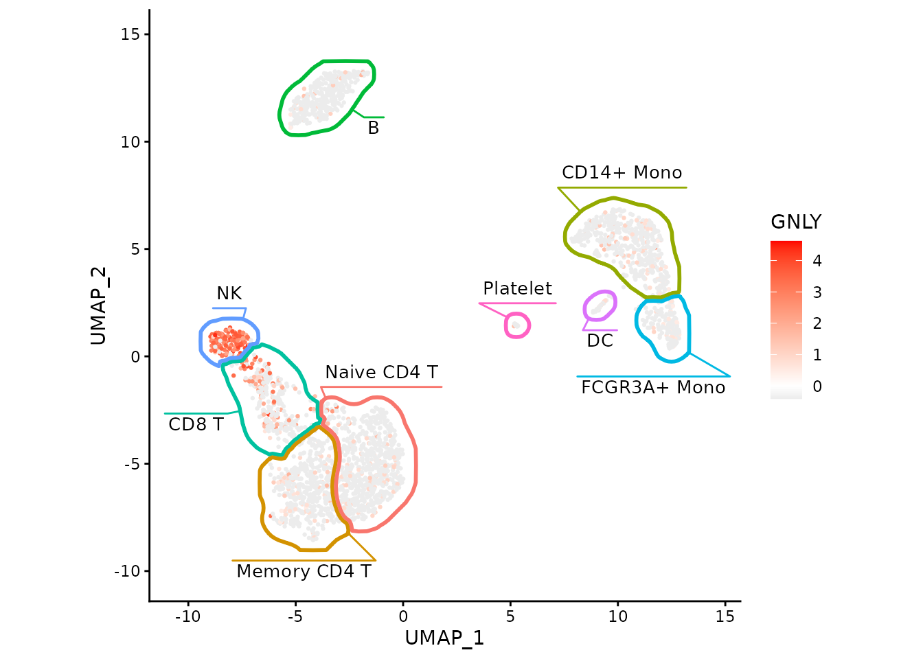
Now we can easily show association between cell types and expression of particular genes, such as GNLY being a good marker for NK cells in this dataset.
ggplot(data, aes(x=UMAP_1, y=UMAP_2)) +
    geom_point(aes(color=GNLY), size=0.5) +
    scale_color_gradient2(low = "#404040", high="red") +
    fancyMask(maskTable, ratio=1, cols = scales::hue_pal()) +
    theme_classic()
We can focus on a single cluster too:
ggplot(data, aes(x=UMAP_1, y=UMAP_2)) +
    geom_point(aes(color=GNLY), size=0.5) +
    scale_color_gradient2(low = "#404040", high="red") +
    geom_path(data=maskTable[cluster=="NK"], aes(group=group)) +
    coord_fixed() +
    theme_classic()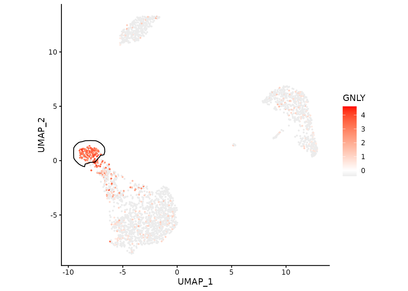
Working with Seurat
For this part of the vignette you need
Seuratpackage.
Let’s get the example PBMC3K dataset:
pbmc3k <- readRDS(url("https://alserglab.wustl.edu/files/mascarade/examples/pbmc3k_seurat5.rds"))
pbmc3k <- NormalizeData(pbmc3k)
pbmc3k
## An object of class Seurat
## 13714 features across 2638 samples within 1 assay
## Active assay: RNA (13714 features, 2000 variable features)
## 2 layers present: counts, data
## 2 dimensional reductions calculated: pca, umapThe same object can be obtained using SeuratData package
(can be installed with
remotes::install_github('satijalab/seurat-data')):
if (requireNamespace("SeuratData")) {
    if (!AvailableData()["pbmc3k", "Installed"]) {
        InstallData("pbmc3k")
    }
    LoadData("pbmc3k")

    pbmc3k <- UpdateSeuratObject(pbmc3k.final)
    pbmc3k
}
Generate masks using a helper function:
maskTable <- generateMaskSeurat(pbmc3k)We can use fancyMask() now, here it reuses colors from
DimPlot automatically:
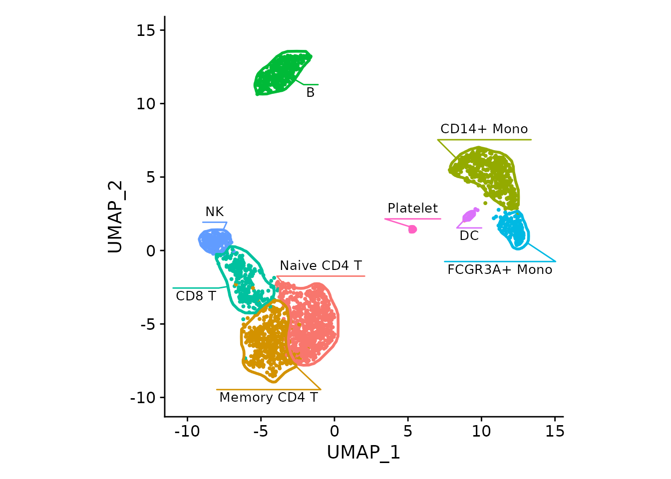
For the DimPlot, the borders can be viewed as redundant
and removed:
Let’s plot an NK cell marker:
FeaturePlot(pbmc3k, "GNLY", cols=c("grey90", "red")) +
    fancyMask(maskTable, ratio=1)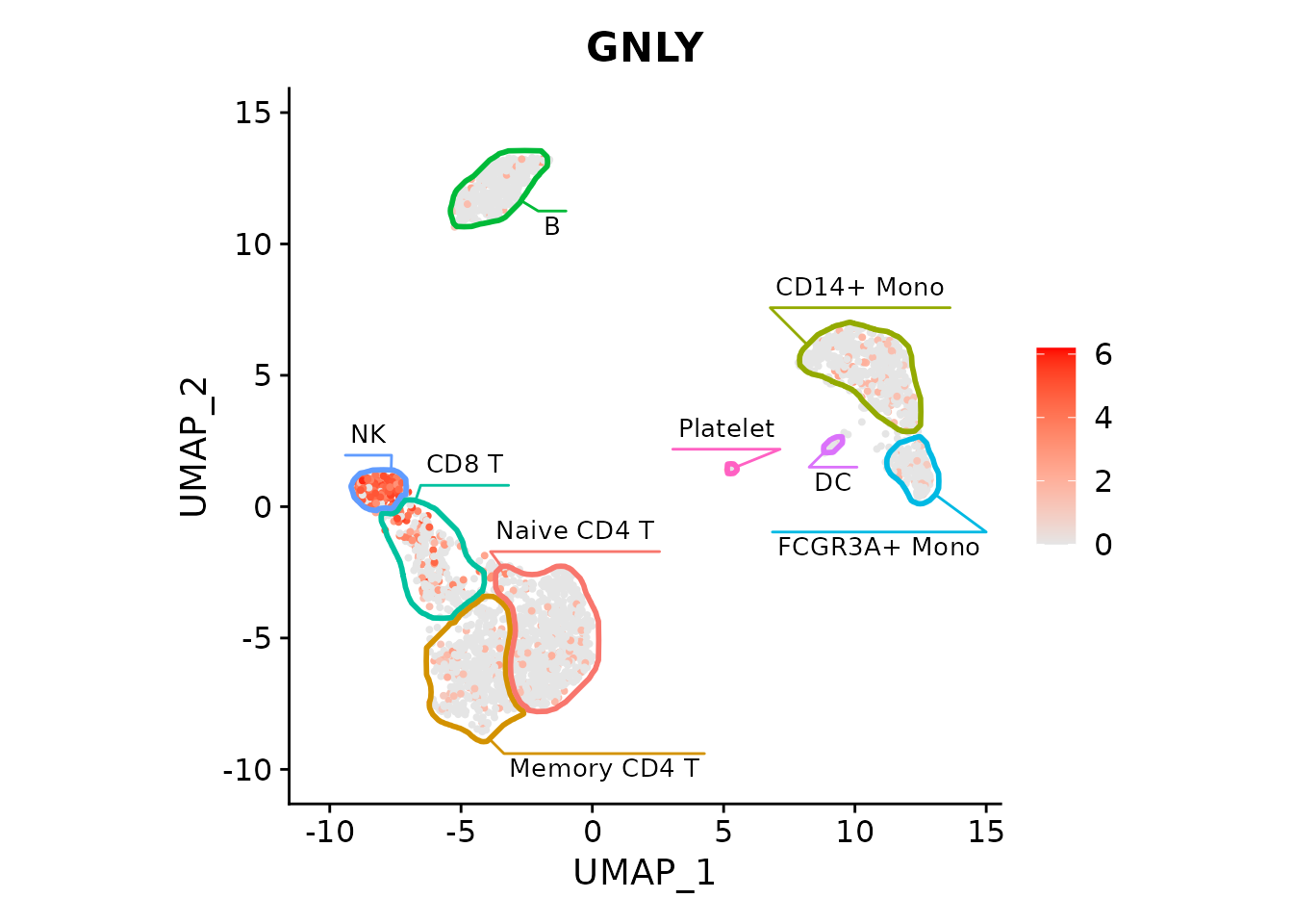
Or multiple markers (skipping the labels to save space, but adding colors):
featureList <- c("MS4A1", "GNLY", "CD3E", "CD14")
FeaturePlot(pbmc3k, features=featureList, cols=c("grey90", "red")) *
    fancyMask(maskTable, ratio=1, linewidth=0.5, label=FALSE, cols = scales::hue_pal())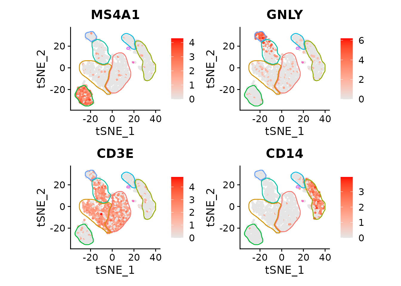
Works with t-SNE too:
pbmc3k <- RunTSNE(pbmc3k)

maskTable <- generateMaskSeurat(pbmc3k, reduction = "tsne")

FeaturePlot(pbmc3k, features=featureList, reduction = "tsne", cols=c("grey90", "red")) *
    fancyMask(maskTable, ratio=1, linewidth=0.5, label=FALSE, cols = scales::hue_pal())
Session info
## R version 4.6.1 (2026-06-24)
## Platform: x86_64-pc-linux-gnu
## Running under: Ubuntu 24.04.4 LTS
##
## Matrix products: default
## BLAS:   /usr/lib/x86_64-linux-gnu/openblas-pthread/libblas.so.3
## LAPACK: /usr/lib/x86_64-linux-gnu/openblas-pthread/libopenblasp-r0.3.26.so;  LAPACK version 3.12.0
##
## locale:
##  [1] LC_CTYPE=C.UTF-8       LC_NUMERIC=C           LC_TIME=C.UTF-8
##  [4] LC_COLLATE=C.UTF-8     LC_MONETARY=C.UTF-8    LC_MESSAGES=C.UTF-8
##  [7] LC_PAPER=C.UTF-8       LC_NAME=C              LC_ADDRESS=C
## [10] LC_TELEPHONE=C         LC_MEASUREMENT=C.UTF-8 LC_IDENTIFICATION=C
##
## time zone: UTC
## tzcode source: system (glibc)
##
## attached base packages:
## [1] stats     graphics  grDevices utils     datasets  methods   base
##
## other attached packages:
## [1] Seurat_5.5.1         SeuratObject_5.4.0   sp_2.2-1
## [4] ggforce_0.5.0        ggplot2_4.0.3        data.table_1.18.4
## [7] mascarade_0.3.4.9000
##
## loaded via a namespace (and not attached):
##   [1] pbapply_1.7-4          deldir_2.0-4           gridExtra_2.3.1
##   [4] rlang_1.2.0            magrittr_2.0.5         RcppAnnoy_0.0.23
##   [7] otel_0.2.0             matrixStats_1.5.0      ggridges_0.5.7
##  [10] compiler_4.6.1         spatstat.geom_3.8-1    reshape2_1.4.5
##  [13] png_0.1-9              systemfonts_1.3.2      vctrs_0.7.3
##  [16] stringr_1.6.0          pkgconfig_2.0.3        fastmap_1.2.0
##  [19] labeling_0.4.3         promises_1.5.0         rmarkdown_2.31
##  [22] ragg_1.5.2             purrr_1.2.2            xfun_0.59
##  [25] cachem_1.1.0           jsonlite_2.0.0         goftest_1.2-3
##  [28] later_1.4.8            spatstat.utils_3.2-3   tweenr_2.0.3
##  [31] irlba_2.3.7            parallel_4.6.1         cluster_2.1.8.2
##  [34] R6_2.6.1               ica_1.0-3              stringi_1.8.7
##  [37] bslib_0.11.0           RColorBrewer_1.1-3     spatstat.data_3.1-9
##  [40] reticulate_1.46.0      parallelly_1.48.0      spatstat.univar_3.2-0
##  [43] scattermore_1.2        lmtest_0.9-40          jquerylib_0.1.4
##  [46] Rcpp_1.1.1-1.1         knitr_1.51             tensor_1.5.1
##  [49] future.apply_1.20.2    zoo_1.8-15             sctransform_0.4.3
##  [52] httpuv_1.6.17          Matrix_1.7-5           splines_4.6.1
##  [55] igraph_2.3.3           tidyselect_1.2.1       abind_1.4-8
##  [58] yaml_2.3.12            codetools_0.2-20       spatstat.random_3.5-0
##  [61] miniUI_0.1.2           spatstat.explore_3.8-1 listenv_1.0.0
##  [64] plyr_1.8.9             lattice_0.22-9         tibble_3.3.1
##  [67] shiny_1.14.0           withr_3.0.3            S7_0.2.2
##  [70] ROCR_1.0-12            evaluate_1.0.5         Rtsne_0.17
##  [73] future_1.70.0          fastDummies_1.7.6      desc_1.4.3
##  [76] survival_3.8-6         polyclip_1.10-7        fitdistrplus_1.2-6
##  [79] pillar_1.11.1          KernSmooth_2.23-26     plotly_4.12.0
##  [82] generics_0.1.4         RcppHNSW_0.7.0         scales_1.4.0
##  [85] xtable_1.8-8           globals_0.19.1         glue_1.8.1
##  [88] lazyeval_0.2.3         tools_4.6.1            RSpectra_0.16-2
##  [91] RANN_2.6.2             fs_2.1.0               dotCall64_1.2
##  [94] cowplot_1.2.0          grid_4.6.1             tidyr_1.3.2
##  [97] patchwork_1.3.2        nlme_3.1-169           cli_3.6.6
## [100] spatstat.sparse_3.2-0  textshaping_1.0.5      spam_2.11-4
## [103] viridisLite_0.4.3      dplyr_1.2.1            uwot_0.2.4
## [106] gtable_0.3.6           sass_0.4.10            digest_0.6.39
## [109] progressr_1.0.0        ggrepel_0.9.8          htmlwidgets_1.6.4
## [112] farver_2.1.2           htmltools_0.5.9        pkgdown_2.2.0
## [115] lifecycle_1.0.5        httr_1.4.8             mime_0.13
## [118] MASS_7.3-65